Distributional Jump Bridges for Disclosure Response Forecasts

What happens when a model reads a company’s SEC filing before predicting how its stock will react, and why the text turns out to say more about risk than about returns.

Disclaimer: Nothing here is investment advice, and none of it was tested as a trading strategy. The study covers 98 large U.S. companies, uses free daily price data rather than intraday trades, and measures returns against SPY (an S&P 500 fund) rather than a full factor model; the result most investors would care about, ranking which stocks will do better, is not statistically reliable. The paper spells out every leakage check behind these numbers.

An 8-K, the form a U.S. public company must file with the SEC whenever something material happens, can move a stock’s price, its trading volume, and how wildly it swings over the following days. Many models that try to forecast these reactions read the filing and the stock’s recent history together and push everything through one shared path to predict every outcome at once; however, there is little reason to think a filing should affect each of those outcomes in the same way. In fact, a filing can clearly change how risky and heavily traded a stock becomes while saying very little about whether it will beat the market. Personally, I believe that difference should be built into the model rather than left for it to discover, because return labels are noisy and it is easy to mistake noise for a signal. I wanted to know whether a model that treats the filing as a nudge to an ordinary forecast, rather than as one more input, would predict market reactions better, and in this experiment it did, although the text helped most with risk, volume, and uncertainty and much less clearly with ranking returns.

Disclosures 101

If you’re already familiar with event studies and probabilistic forecasting, feel free to skip to The Real Stuff.

As always, let’s call on our friends Alice, Bob, and Charlie. Alice runs a small forecasting desk at a local newspaper, and every week she predicts three things about each restaurant in town: how much its sales will beat the town’s average, how much more unpredictable its week will be than usual, and how much more crowded it will get. She makes these forecasts from each restaurant’s recent numbers alone, and she always gives a range along with her best guess, since some weeks are simply harder to call than others.

Restaurants also send out announcements, like a new chef, a failed health inspection, or a change in hours, and Bob’s job is to read them. The simplest way to use Bob would be to hand him Alice’s numbers and the announcement and let him rewrite the forecast from scratch. Charlie, the editor, prefers a stricter arrangement: Alice makes her ordinary forecast first, as if nothing had been announced, and Bob may only nudge it, by a limited amount, and widen or narrow its range. In a more cautious version of the desk, Charlie adds one more rule, under which Bob may adjust the crowding and unpredictability forecasts but must never touch the sales forecast, since that is the number most easily fooled by a lucky guess.

To keep Bob honest, Charlie also has the desk forecast each restaurant on a quiet week with no announcement at all, and Bob is penalized for nudging anything on those weeks. Furthermore, every forecast must be made using only numbers from before the announcement went out, and Charlie checks every timestamp to make sure no one peeked at the following week. At the end of the season, the desk is judged two ways: by how close its forecasts came, and by whether the restaurants it expected to beat the average actually ranked near the top. Because one large restaurant could dominate the second score, Charlie checks it restaurant by restaurant, asking whether the ranking would hold up if any single restaurant were dropped.

Finally, to learn whether Bob is actually helping, Charlie can tear out Bob’s nudges entirely, hand Bob blank announcements, or shuffle the announcements so that each restaurant gets someone else’s. If the forecasts get worse in each case, then Bob, and the specific words he read, were doing real work.

The Real Stuff

Every part of the forecasting desk corresponds to a piece of the model and its evaluation:

• Restaurants → Firms
  • The panel covers 98 large U.S. companies, observed from 2020 to 2025.
• Announcements → 8-K Filings
  • There are 7,236 filings, read straight from the SEC’s public EDGAR records.
  • Each filing’s text is turned into a vector $e$ by BGE-small, a general-purpose text encoder.
• Three Forecasts → Targets
  • The abnormal return is the firm’s return minus SPY’s over the five sessions after the filing¹.
  • The volatility jump is how much more the stock’s daily returns swing in that window than in the 20 sessions before it.
  • The volume jump is how much heavier its trading is than before.
• Alice’s Forecast → No-Event Distribution
  • A recurrent network (a GRU) reads the 40 trading days before the filing and predicts a Gaussian for each target, with a mean \(\mu_0\) and a log-variance \(\ell_0\).
• Bob’s Nudges → Disclosure Bridge
  • The filing’s embedding produces bounded shifts \(\Delta\mu\) and \(\Delta\ell\) that move the means and the uncertainty.
• Charlie’s Rule → RC-DJB
  • The return-conservative variant fixes \(\Delta\mu_{\text{return}} = 0\), so text may move volatility, volume, and uncertainty but never the return forecast itself.
• Quiet Weeks → Matched Controls
  • Each filing gets one control date for the same company, away from any known event, and the bridge is penalized for moving on those dates.
• Timestamps → Leakage Guard
  • Every feature comes from strictly before the window starts, training uses dates through 2023, validation uses 2024, and testing uses what came after.
• Closeness → MSE
  • Mean squared error across the three targets, averaged over the 2,463 held-out rows.
• Ranking → Rank IC
  • The Spearman correlation between predicted and realized abnormal returns, where 0 means the ordering is no better than chance.
• Per Restaurant → Clustered Intervals
  • Confidence intervals resample whole companies rather than individual filings, and a leave-one-ticker-out check drops each company in turn.
• Tearing Out Bob → Interventions
  • Removing the bridge, zeroing the text, or shuffling it across rows shows how much the bridge and the text actually contribute.

With those pieces in place, the whole model can be written as Alice’s forecast plus Bob’s nudge:

together with a matching nudge \(\ell_1 = \ell_0 + \Delta\ell\) to how unsure the forecast is. The full Distributional Jump Bridge (DJB) lets Bob nudge all three means, while RC-DJB holds the return entry of \(\Delta\mu\) at zero.

No Peeking

In financial forecasting, the most common way to fool oneself is to let the future leak into the inputs, so the data pipeline was built around that risk first. Each filing’s timestamp comes from the SEC’s own acceptance time, and a filing accepted before the 4:00 p.m. close starts its window that same day, while one accepted after the close (or on a non-trading day) starts on the next trading day. Every row was then checked to make sure its latest feature date came strictly before its window began, and none failed.

The split is also strictly chronological, with 9,729 training rows through 2023, 2,280 validation rows from 2024, and 2,463 held-out rows after that, so that no model is ever tuned on data from its own future. Against that held-out year, I compared DJB and RC-DJB with five baselines:

• No-Event
  • Alice alone, trained on the same rows but without any text.
• Concat Fusion
  • The filing’s text and the market history are simply joined and pushed through one shared predictor.
• Event Bottleneck
  • The text passes through a small stochastic bottleneck before predicting the targets.
• Disclosure Operator
  • The text acts through a low-rank operator on the market state.
• Event-Jump SSM
  • A state-space model in which the text causes a jump in the hidden state.

Closest Forecasts

On the held-out year, DJB had the lowest error of every model, with a multi-target MSE of 0.0552. That may not sound like much on its own; however, the paired comparisons, which resample the same rows for both models, show that it beat every baseline by more than chance. In fact, it improved on concat fusion, the usual way of combining text with market data, by 0.0114, a reduction of about 17%, and it edged out the closest competitor, the event-jump state-space model, by a smaller 0.0014. DJB also had the highest point estimate for Rank IC, at 0.0330.

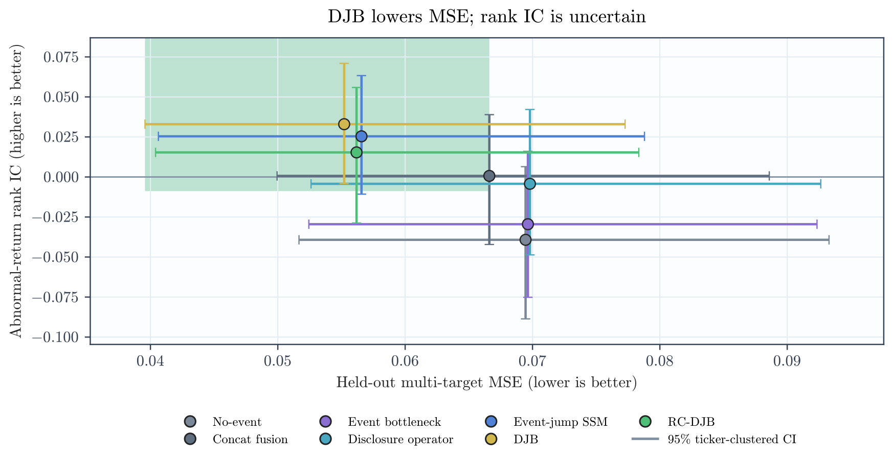Each point is one model on the held-out year, with error on the horizontal axis (lower is better) and return ranking on the vertical axis (higher is better). DJB sits furthest toward the upper left, but every model’s ranking interval reaches zero or below.

The baselines also show what this result does not mean. The no-event model on its own had the worst ranking of the group (a Rank IC of -0.0393), which does not mean that market history is useless; it means only that Alice, working alone, cannot explain what happens after a filing. Thus, the gain comes from routing the text through Bob’s nudges on top of her forecast, not from either part by itself.

Shaky Rankings

The ranking result is the weakest part of the paper, and it deserves to be read as such. DJB’s Rank IC of 0.0330 has a ticker-clustered interval running from -0.0042 to 0.0710, which means that once uncertainty is measured company by company, the ranking signal cannot be distinguished from zero². The leave-one-ticker-out check is more encouraging, since dropping any single company still left DJB’s Rank IC positive, from a low of 0.0263 (without KLA) to a high of 0.0381 (without Costco). As such, no one company is carrying the result, even if the result itself is small.

The ranking also depends on settings in ways that make me cautious. Loosening the temperature on the ranking loss from 0.02 to 0.10 cut DJB’s Rank IC roughly in half, to 0.0152, while it nudged RC-DJB’s up from 0.0154 to 0.0201, and in every case the clustered interval crossed zero. Additionally, the month-by-month Rank IC swung widely, and predicted deciles did not line up into a clean staircase of realized returns. Thus, there is some ordering information here, but not the kind of large, steady effect that anyone should build on.

Charlie’s Rule

RC-DJB, the cautious desk, is less a competitor than a controlled experiment, since it asks what is lost when the text can no longer move the return forecast. Its error was slightly higher than DJB’s (0.0562 against 0.0552, a gap of 0.0010 that was nonetheless reliable), and its Rank IC was about half of DJB’s, at 0.0154. In exchange, its probabilistic forecasts were very slightly better, with a Gaussian negative log-likelihood of -2.2961 against DJB’s -2.2815. The unconstrained bridge, then, is the better point forecaster in this sample, while the constrained one makes it possible to see exactly what the text does when it cannot touch returns.

The interventions show that it still does a great deal. Tearing out the bridge raised RC-DJB’s error on filing rows by 0.0183, and its negative log-likelihood on those rows jumped from -2.22 to 4.81, which means that Alice’s forecast alone is badly calibrated for filing weeks. Zeroing the text raised the error by 0.0037, and shuffling it across filings raised it by 0.0025, so the specific words matter and not just the presence of a filing. All of this happened while the return forecasts did not move at all, which is exactly what Charlie’s rule guarantees.

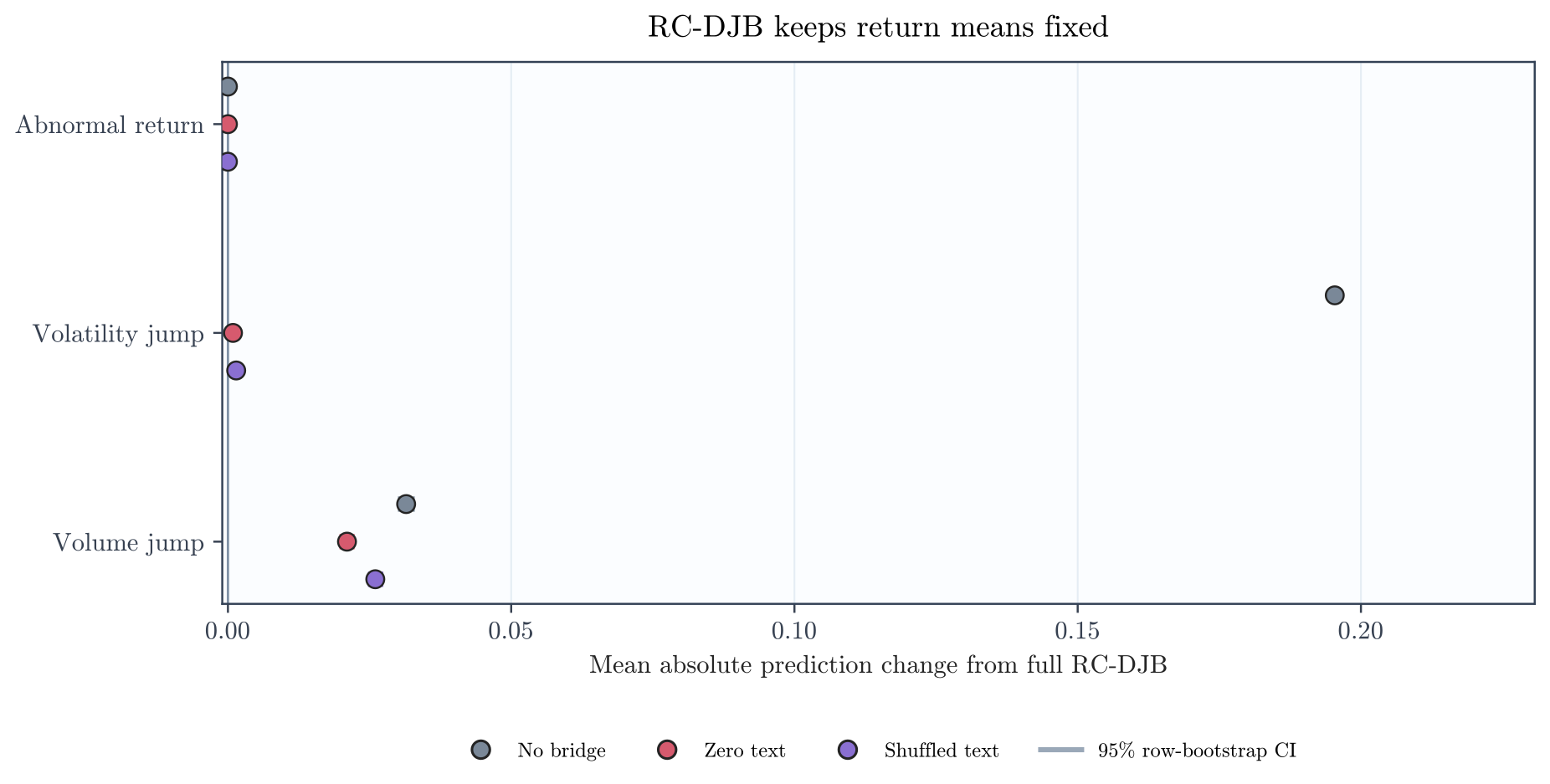How far RC-DJB’s predictions move under each intervention. The abnormal-return forecast stays exactly fixed, while removing the bridge moves the volatility forecast a long way and every intervention moves the volume forecast.

There is one caveat, which is that Charlie’s rule protects the return mean but not the return uncertainty. RC-DJB’s nudges to the return log-variance still carried a little ranking information (a signed Rank IC of 0.0274), so the rule blocks the text from moving return forecasts directly without fully isolating the return distribution from it.

Where Bob Works

Looking at each target separately shows where the bridge actually acts. In RC-DJB, the volatility nudges were large on filing rows and on quiet control rows alike (about 0.198 and 0.193), so on average the volatility channel moves almost as much on a quiet week as on a filing week. The volume nudges, on the other hand, were roughly four times larger on filings than on controls (0.052 against 0.012), which makes volume the channel where the text most clearly responds to the fact that something happened.

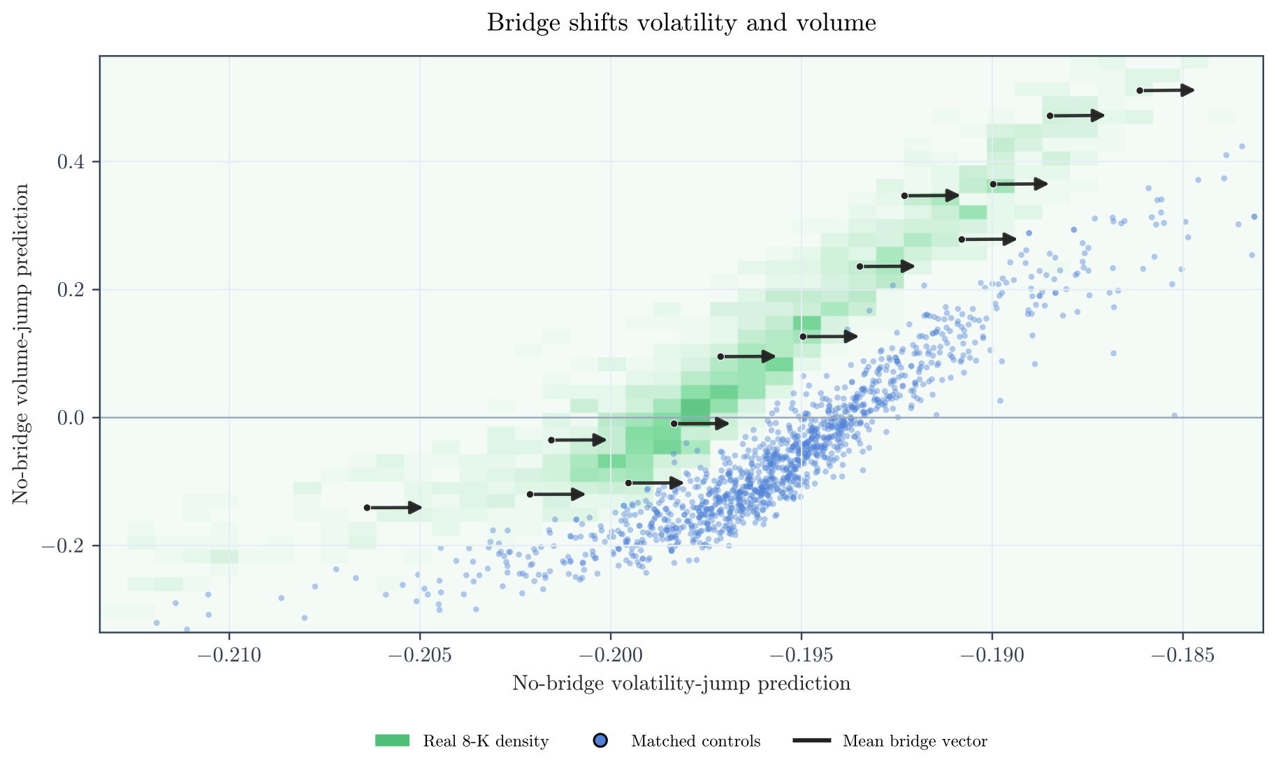Real filings (green density) and matched controls (blue points) in the plane of Alice’s volatility and volume forecasts, with arrows showing the direction of the bridge’s average nudge in each region. The arrows are drawn at a fixed scale to show direction and relative strength, not true length.

Volume Leads

The bridge is also far from a uniform offset applied to every filing. Sorting held-out filings by how much the bridge moved them shows that the volatility nudge stays nearly flat across all ten deciles, while the volume nudge grows steadily, from almost nothing to about 0.13. In fact, the filings with the strongest nudges were also the ones that went on to see the largest realized changes in volume and volatility, which fits decades of event-study work showing that the market’s reaction depends on the filing, the firm, and the moment.

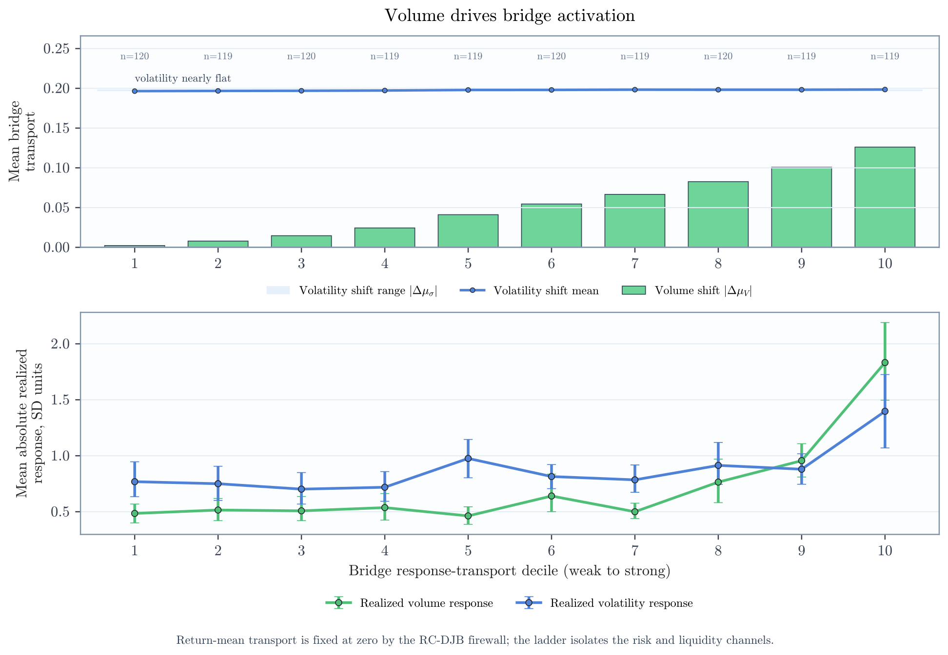Held-out filings sorted into deciles by how strongly RC-DJB’s bridge moved them. Top: the volatility nudge (line) is nearly constant while the volume nudge (bars) climbs. Bottom: the realized volume and volatility responses rise sharply in the strongest decile.

So What?

• Routing Matters
  • Treating a filing as a bounded nudge to an ordinary forecast beat simply joining its text with market data.
  • The same text representation fed every text-aware model, so the gain comes from the architecture rather than the encoder.
• Risk Before Returns
  • In this experiment, disclosure text helped most with volatility, volume, and uncertainty.
  • Its effect on return ranking was positive but not statistically reliable.
• Audit the Ranking
  • A ranking statistic should be reported with intervals that resample whole companies, along with a leave-one-company-out check.
  • Without them, a small and unstable signal is easy to oversell.
• Constraints as Tests
  • A rule like Charlie’s is useful less as a better model than as a way to see exactly what the text does when one path is blocked.

Final Notes

• Large-Cap Panel
  • The 98 companies are large and heavily traded, not a broad market.
  • Small, illiquid, or more varied samples are the obvious next test.
• Daily Data
  • Prices are free daily closes rather than intraday trades, so the return target measures drift over the following days rather than the immediate jump.
  • Returns are measured against SPY rather than a full factor model.
• General Encoder
  • BGE-small is a general-purpose encoder, and a finance-specific or long-document model could change the absolute numbers.
• No Trading Test
  • Nothing here accounts for spreads, commissions, market impact, borrowing limits, or turnover³.
• Not Causal
  • Charlie’s rule is an architectural constraint on predictions, not a causal estimate of what filings do to markets.
• One Seed
  • Every model was trained once with the same fixed seed, so run-to-run variation is not measured.

As always, if you’ve read this far, thank you! My hope is that more models of market reactions start asking which outcomes a piece of text should be allowed to change, rather than letting it change everything at once. The full paper, with the loss terms and every diagnostic table I only summarized here, is available here, and the code (along with the data-ingestion scripts and leakage tests) is on GitHub. If you work on financial forecasting or event studies and have thoughts, I’d love to hear them.

If you’d like to cite this:

@misc{gupta2026djb,
  title  = {Distributional Jump Bridges for Disclosure Response Forecasts},
  author = {Gupta, Aryan},
  year   = {2026},
  url    = {https://aryan-cs.github.io/distributional-jump-bridges/djb.pdf}
}