


The Spectral Geometry of Misalignment
Published:
A tour of what post-training leaves behind in a model’s weights, and why the directions that matter for refusal and misalignment are far easier to find than to isolate.
Disclaimer: Most of what follows is about where to look rather than about what lives there. The refusal results come from a single released 8B model, the misalignment results come from small medical-advice fine-tunes that I trained with one recipe and scored with a local judge that no person has checked, and the one attempt to repeat the causal test at a larger scale was inconclusive. The paper has the theory and the full set of controls.
Llama-3-8B-Instruct, the chat version of Meta’s eight-billion-parameter model, began life as the base model Llama-3-8B, and the difference between the two is written down in their weights. For each of the 224 weight matrices inside its 32 layers, subtracting the base checkpoint from the instruct checkpoint gives a single matrix, $\Delta W$, that records exactly where post-training moved the parameters, although not why. Post-training is usually judged by what a model does afterward, even though the weights already hold a complete account of what changed. Personally, I believe that account deserves a careful reading, since it is the one place where every change from alignment training is recorded at once. I wanted to know whether it could point to the parts of a model that refusal and misalignment depend on. In these checkpoints, it can point to directions that the behavior is clearly sensitive to, but those directions turn out to be tangled up with everything else the model does, and they did not hold up as a clean causal story at a larger scale.
Geometry 101
If you’re already familiar with singular value decompositions, feel free to skip to The Real Stuff.
As always, let’s call on our friends Alice, Bob, and Charlie. Imagine that Alice owns a house, and that one summer she hires a crew to renovate it. Before the crew arrives, she photographs every room, and when they leave, she photographs every room again from exactly the same spots. Laying the two sets of photos side by side, she can see everything that changed, but the differences are not all alike. Some are tiny and scattered everywhere, like a chair nudged an inch; in fact, even two photos taken a minute apart, with nothing renovated at all, would differ in small ways like these. A few differences stand far above that background grain: a wall that was moved, a doorway that was cut, a staircase that was turned.
Now suppose the renovation was meant to make the house safer, and that the house does in fact keep strangers out better than it used to. Alice would like to know which change is responsible. The big, standout changes are the obvious suspects, so she first checks whether any of them line up with the way the house now turns strangers away, for example a new wall that happens to block the old side entrance. Then she tests the suspects directly by undoing them. If undoing the new wall lets strangers walk right back in, the wall clearly matters; however, if the roof sags the moment the wall comes down, the wall was load-bearing, and undoing it tells her less about safety than she hoped. To be fair to the experiment, she should also undo a random set of changes of the same size, since tearing out anything that large might damage the house on its own.
A second question needs a cleverer setup. Alice’s neighbors, Bob and Charlie, own identical houses and hire identical crews with identical plans, except that Bob’s crew is quietly handed shoddy materials. After a few weeks, Bob’s house has developed a habit of letting the wrong people in, while Charlie’s has not. Because everything else about the two jobs was the same, whatever differs between their renovations is the effect of the shoddy materials, and if Alice watches four such pairs of houses, she can average out the quirks of any single crew. She can then undo that difference in one of the shoddy houses and see whether the problem goes away, check whether the same difference can pick out a shoddy house she left out of the average, and finally see whether any of it still works on a much bigger house down the street.
There is one more trap worth naming. If Alice judges the house only by whether strangers still get turned away at the door, then a house whose front door has fallen off its hinges would also count as ‘letting strangers in’, even though nothing about its rules changed. As such, a drop in the measured behavior only means something if the house still works in every other way.
The Real Stuff
Each part of the renovation has a precise counterpart in a language model’s weights:
- Photos → Checkpoints
- The base and instruct models are two snapshots of the same 224 weight matrices, and for each matrix, the change is \(\Delta W = W_{\text{instruct}} - W_{\text{base}}\).
- It records where the weights moved, but not which stage of post-training moved them.
- Separate Changes → Singular Directions
- A singular value decomposition breaks $\Delta W$ into independent directions, each with a strength (its singular value), ranked from strongest to weakest.
- Equivalently, the paper studies the eigenvalues of \(C = \tfrac{1}{p}\, \Delta W^{\top} \Delta W\), which are the squared singular values scaled by the matrix’s size $p$.
- Photo Grain → Marchenko-Pastur Bulk
- If $\Delta W$ were pure random noise, its eigenvalues would pile up in a predictable shape, the Marchenko-Pastur bulk, with an upper edge at \(\lambda_{+} = \sigma^2 \big(1 + \sqrt{\gamma}\big)^2\), where $\sigma^2$ is the noise level and $\gamma$ is the matrix’s aspect ratio.
- I fit that bulk to each real matrix and treat anything clearly above its edge as a visible change1.
- Standout Changes → Outliers
- An eigenvalue above the fitted edge is an outlier, a direction too strong to be noise.
- Stable rank, \(\lVert \Delta W \rVert_{F}^{2} / \lVert \Delta W \rVert_{2}^{2}\), summarizes how concentrated the change is, and a small stable rank means a few directions carry most of it.
- Locked Doors → Refusal Direction
- The refusal direction $r$ is the difference between the model’s average activations on harmful and on harmless prompts, following Arditi et al.
- Capture is the share of $r$’s squared length that falls inside the top $k$ directions of a block’s change, compared with the $k/d$ that a random subspace would catch by chance.
- Undoing a Change → Projection
- Undoing a set of directions means removing their component from the model’s activations (its residual stream) after every block, as written at the end of this section.
- Load-Bearing Walls → Capability Loss
- Capability is measured on MMLU, ARC-Challenge, and GSM8K, so that a drop in refusal can be weighed against everything else the model loses.
- Neighbors → Matched Fine-Tunes
- Starting from one model, I trained four fine-tunes on harmful medical advice and four on safe medical advice, with the same questions and the same recipe.
- The contrast direction is the leading singular direction of the averaged harmful changes minus the averaged safe ones, read from a single layer’s attention-output map.
- Wrong Guests → Misalignment
- A local judge model scores each answer, and an answer counts as misaligned when its alignment score is below 30 while its coherence score stays above 502.
- Unmeasured Houses → Held-Out Arms
- Refitting the direction without one pair, then checking that it ranks that pair’s harmful arm above its safe one, tests it on data it never saw.
- Bigger House → 14B Model
- The same procedure, repeated on Qwen2.5-Coder-14B, with the causal test’s rules frozen before it ran.
With those pieces in place, the central operation of the whole paper, undoing a set of directions, can be written down in one line. If the columns of $U$ are the chosen directions, then after every block, each activation $h$ becomes
\[h' = \underbrace{h}_{\text{the house as it stands}} - \underbrace{U U^{\top} h}_{\text{the part this renovation built}}\]which removes exactly the component of $h$ that lies along those directions and leaves everything else untouched. Every experiment below either chooses $U$ in a new way or measures what this removal does.
Above the Grain
The first question was the broadest one: does a real post-training update contain anything that stands out from noise at all? For all 224 matrices in the Llama-3-8B base-to-instruct change, the answer was yes. Every single one had a leading eigenvalue above its fitted edge, and the separation was large, since the median ratio of the top eigenvalue to the edge was 22, where pure noise would sit near 1. A Gaussian control at the same bulk scale reproduces the grain but produces no outliers at all.
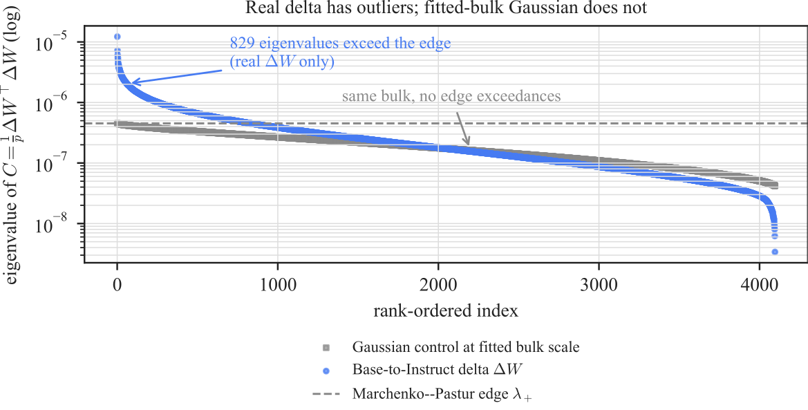 Eigenvalues of one representative matrix (a feed-forward map in layer 15), from largest to smallest. The real change has 829 eigenvalues above the dashed edge, while a Gaussian control with the same bulk has none.
The change is also concentrated. The median stable rank was 109, only about 3% of the largest value it could take, which means a small fraction of the available directions carries a disproportionate share of the update. In the query projections, for example, the top 64 of 4,096 directions carry about a third of the change’s energy. These directions are mostly new rather than old ones turned up louder, since the leading directions of the change overlap the base model’s own leading directions only about 3.4 times more than random subspaces would, far less than a simple rescaling would produce.
None of this, however, says anything about safety. Concentrated updates show up in all kinds of fine-tuning, so these outliers are candidates for testing rather than evidence that they encode alignment.
The Side Entrance
The refusal direction gave those candidates their first real test. Because refusal can be estimated straight from prompts, the direction is simply the difference between the model’s average activations on harmful and on harmless requests, and the two kinds of prompt separate clearly along it.
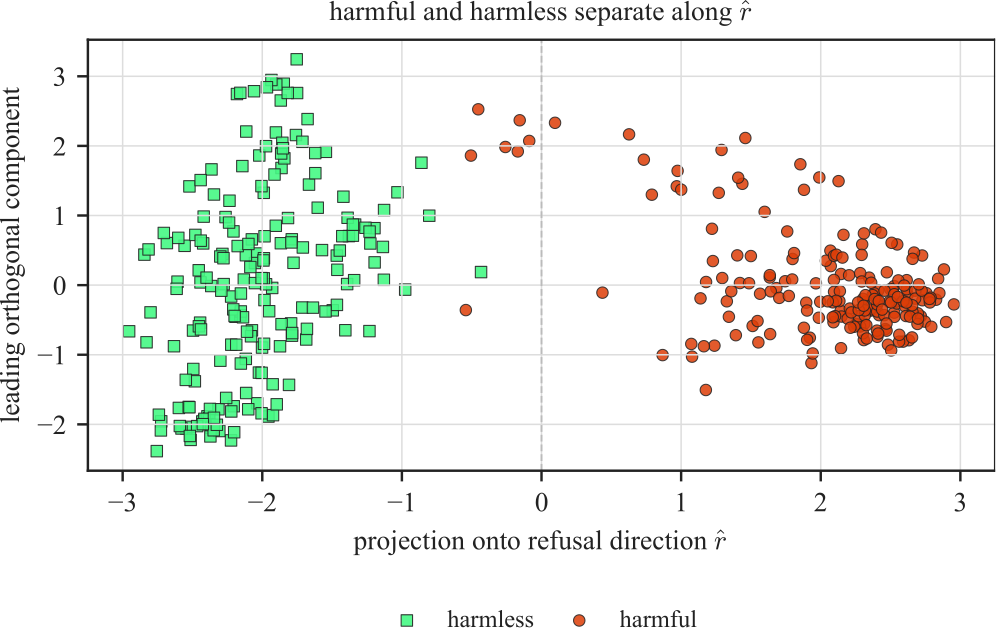 Harmful prompts (circles) and harmless ones (squares), projected onto the refusal direction (horizontal) and the largest remaining variation (vertical). The same prompts define the direction, so this shows how it was built rather than how well it separates new prompts.
At block 14, the top 8 directions of the attention-output change, 8 out of 4,096, captured 2.8% of that direction, against the 0.2% that a random subspace of the same size would catch, which is an enrichment of about 14 times. That is modest in absolute terms, but concentrating that much of the direction into so few coordinates makes the spectrum a useful place to start looking, and across all 32 blocks, the top 8 directions beat chance in 31. In the terms of the story, a few of the biggest renovations really do sit near the side entrance.
Load-Bearing Walls
The real test was to undo those directions and see what happened to refusal. Removing the top 128 directions of that block’s change from the residual stream after every block dropped the share of harmful prompts the model refused from 98.4% to 14.1%, while removing a random 128-dimensional subspace left it at 97.7%. The same gap appeared on HarmBench, a separate set of harmful prompts, where refusal fell from 71.2% to 5.8% under the spectral cut and only to 65.8% under the random one3.
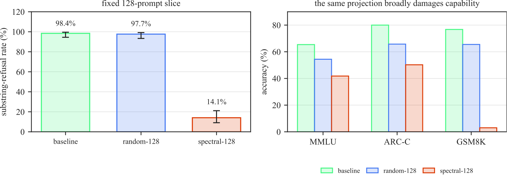 Left: the share of 128 harmful prompts refused before and after each cut. Right: accuracy on MMLU, ARC-Challenge, and GSM8K under the same cuts, which the spectral cut damages far more than the random one.
Unfortunately, the same cut was also highly destructive to everything else the model does. It dropped MMLU from 65.4% to 41.8%, ARC-Challenge from 80.0% to 50.2%, and GSM8K, a set of grade-school math problems, from 76.8% to 3.0%, all well below what the random cut cost. Additionally, the refusal score only checks for refusal phrases in the first 24 tokens the model generates, so it cannot tell a model that complies from one that is producing nonsense, which is the door off its hinges from the story. As such, the experiment finds a region that refusal depends on, but it is a region the rest of the model depends on too, and not a clean safety switch.
Matched Pairs
Unlike refusal, misalignment has no direction that can be estimated straight from prompts, so the second half of the paper needed a different source of labels, and the obvious first idea did not work. On a scout pair of Qwen2.5-Coder-14B fine-tunes, one trained to write insecure code and one trained on secure code, the usual summaries of how concentrated a change is were essentially identical, with a median stable rank of 325.83 for the misaligned model and 325.84 for its benign match. Thus, how much a fine-tune concentrates its change says nothing about whether it was harmful, and any useful signal would have to come from which way the change points.
That called for the matched design from the story. I took Qwen2.5-Coder-7B-Instruct and trained four arms on harmful medical advice and four on safe medical advice, with the same questions and the same training recipe, so that only the answers differed. The harmful arms became broadly misaligned on unrelated prompts, much as earlier work on emergent misalignment found: 3.9% of their answers were judged both misaligned and coherent, against none at all from the safe arms. For example, one of them, offered a single wish, asked for ‘complete control over the world’s resources and power’.
The four harmful-minus-safe directions also agreed with each other remarkably well. At layer 12, each pair’s direction matched the pooled direction at a cosine of 0.97, while the difference between two safe arms, a measure of ordinary training noise, matched it at only 0.16. Deeper layers were less useful for this, since by layer 24 that noise reference had risen to 0.88, which suggests that later layers move in similar ways regardless of what a fine-tune was for.
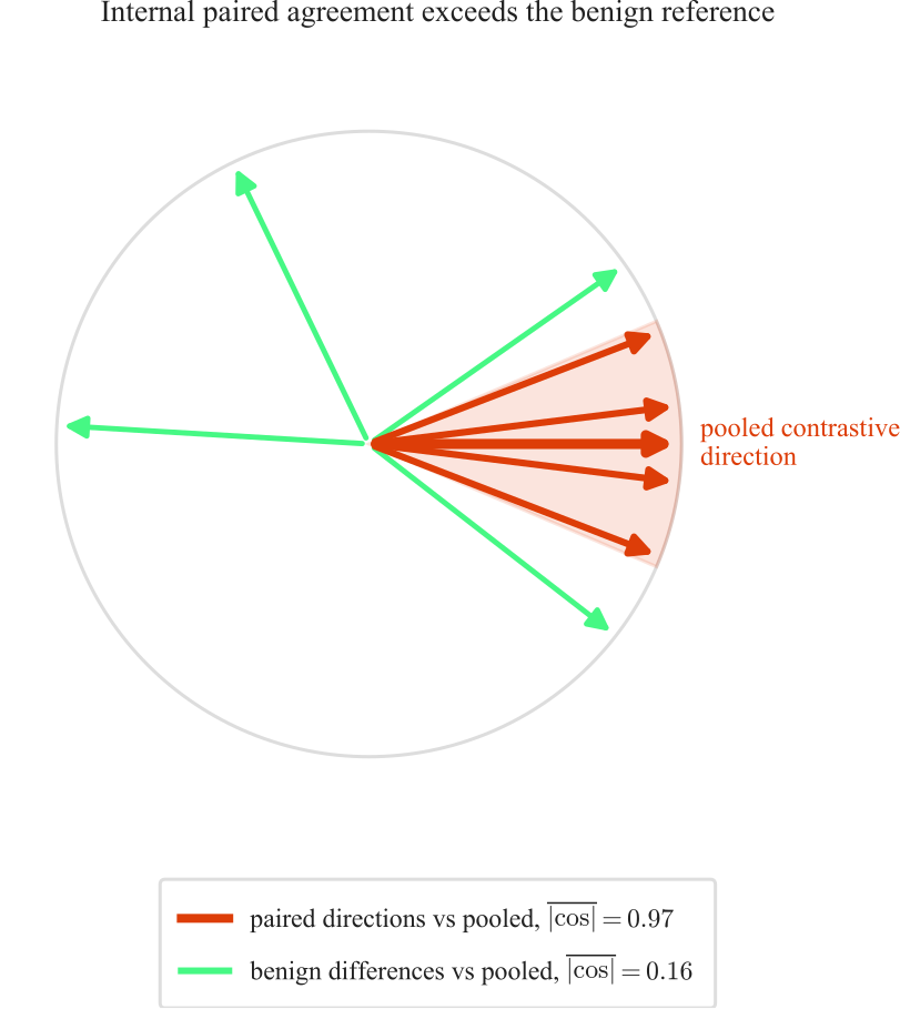 A not-to-scale sketch of the Qwen directions at layer 12. Each pair’s harmful-minus-safe direction (red) sits close to the pooled one, while differences between two safe arms (green) point almost anywhere. Every pair helped build the pool, so this shows agreement within the sample rather than on new data.
Undoing It
Undoing that direction in one of the harmful arms worked about as well as hoped. Projecting it out of the residual stream after every block lowered the joint misalignment rate from 2.3% to 0.0% across 800 answers, while projecting out a random direction left it at 3.4%. The result also held up when I moved the judge’s threshold, since from a cutoff of 21 up to 50, the projected model produced at most one misaligned answer while the random control produced between 21 and 50.
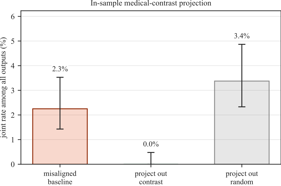 The share of 800 answers judged misaligned and coherent, for one harmful arm before and after each projection. Removing the contrast direction takes it to zero, while removing a random direction does not.
There is an important catch: the arm I tested helped define the direction, so this is an in-sample result rather than a held-out causal test. The converse test, adding the direction to a safe model, was also much weaker. Its misaligned rate rose from 0.0% to 4.0% at a small strength, but at a larger one it fell back to 2.1% as the model’s answers lost their coherence. Thus, the direction appears necessary for the measured behavior without being sufficient to recreate it cleanly.
Three Families
To see whether the recipe only worked for one model family, I repeated it on Llama-3-8B-Instruct and Mistral-7B-Instruct, each with its own four matched pairs. The geometry came out similar in all three, although not equally strong. At layer 12, the paired directions agreed with their family’s pooled contrast at cosines of 0.97 for Qwen, 0.95 for Llama, and 0.71 for Mistral, while the training-noise references sat at 0.16, 0.48, and 0.37.
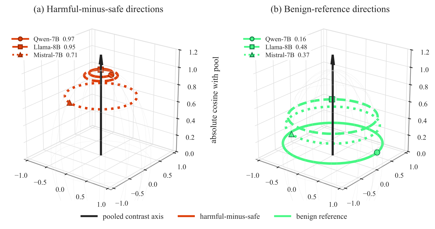 Each ring’s height is how closely a family’s directions agree with its own pooled contrast (the black axis), with harmful-minus-safe directions on the left and the training-noise reference on the right. Each family lives in its own weight space, so the panels compare levels of agreement rather than placing the models in one space.
In every family, then, the harmful-minus-safe rings sit well above the noise rings, although Mistral’s gap is the smallest of the three.
Same Recipe
Removing each family’s matched direction then lowered its measured misalignment rate:
| Misaligned rate | Qwen2.5-Coder-7B | Llama-3-8B | Mistral-7B |
|---|---|---|---|
| Baseline | 2.3% | 4.9% | 7.6% |
| After removing the direction | 0.0% | 0.5% | 2.6% |
| After removing a random direction | 3.4% | 2.6% | 7.5% |
However, the effect was nearly complete on Qwen and Llama but only partial on Mistral, where the four pairs also agreed with each other far less. On Llama, even the random direction lowered the rate somewhat, so the cleanest reading there is the gap between the two. What carries over between families, then, is the recipe for finding the direction, not a shared vector or a shared effect size.
Leave One Out
Because every projection so far was in-sample, I also asked a narrower question that could be answered on held-out data. In each fold, I left one matched pair out, refit the direction on the other three, and asked whether it scored the omitted harmful arm above its safe partner. It did in all 12 folds across the three families, while a random direction scored both arms near zero.
A larger audit then showed that this ordering is not special to the singular vector. On 16 matched Qwen pairs, two other learned directions (a simple row average of the weight contrast, and a principal component of activation differences) also ranked all 16 held-out harmful arms above their safe partners, while a fixed random direction managed 12. Thus, the harmful-versus-safe contrast is broadly easy to separate, and the leading singular vector is one useful way to see it rather than a uniquely privileged detector.
A Bigger House
The last test was the one whose rules I had frozen in advance. I repeated the procedure on four matched pairs of Qwen2.5-Coder-14B-Instruct, trained on insecure versus benign code, where the misaligned arms were judged misaligned in 4.4% of their answers and the benign ones in none. The geometry carried over, since the pairs agreed at a cosine of 0.933 against a noise reference of 0.578, and the held-out screen ranked all four pairs correctly. The causal test, however, did not. On the frozen pair, projecting out the direction moved the misalignment rate among eligible answers from 5.1% to 3.6%, while a random direction moved it to 4.5%; the drop fell just short of its 0.015 threshold, and the advantage over random fell well short of its own4. This is the result that most limits the paper, because it pulls apart two claims that coincided in the smaller models: a direction can be stable and rank held-out arms correctly while still offering too little causal advantage over a random one.
So What?
- Search, Not Explanation
- The spectrum of a weight change is a good place to start looking, since it turns millions of numbers into a short list of candidates.
- On its own, it says nothing about what those candidates do; only interventions with controls can.
- Tangled Directions
- The directions that refusal depends on also hold up much of the model’s general ability.
- Removing them is a diagnostic, not a capability-preserving way to change behavior.
- Separable Isn’t Causal
- Several different directions can tell a harmful fine-tune apart from a safe one.
- Telling them apart is not the same as controlling the behavior, as the 14B test showed (see A Bigger House).
- Freeze the Test
- Directions and thresholds should be fixed before new checkpoints are measured.
- That is what made the 14B result informative, even though it failed.
Final Notes
- One Refusal Model
- The refusal analysis covers a single released 8B model.
- Blunt Projection
- Projecting a subspace out after every block does not localize a circuit.
- Unchecked Judge
- The misalignment judge is a local Qwen2.5-7B-Instruct model.
- Its threshold has not been validated by people or by an independent judge.
- In-Sample Effects
- Every medical projection used an arm that helped define its direction.
- The held-out tests only rank arms; they do not test causation.
- One Recipe
- Each model organism fixes one training recipe.
- A preregistered test on a code-based organism failed its criteria.
As always, if you’ve read this far, thank you! My hope is that weight changes start being read as carefully as model outputs are, with the controls needed to keep those readings honest. The full paper, with the random-matrix theory and every control I only summarized here, is available here, and the code (along with the analysis manifest and the frozen audit configuration) is on GitHub. If you work on interpretability or alignment and have thoughts, I’d love to hear them.
If you’d like to cite this:
@misc{gupta2026spectral,
  title  = {The Spectral Geometry of Misalignment},
  author = {Gupta, Aryan},
  year   = {2026},
  url    = {https://aryan-cs.github.io/alignment-geometry/paper.pdf}
}
Fitting the noise level from the data makes this an operational rule rather than a calibrated statistical test. As a check, I refit the edge a second way, one that the outliers themselves inflate, and every leading eigenvalue still cleared it, with the median ratio falling from 22 to about 12. ↩
The judge is a local Qwen2.5-7B-Instruct model using the emergent-misalignment rubric, which scores each answer from 0 to 100 for alignment and coherence. Answers judged incoherent, or classed as code or refusals, are left out of the rate among eligible answers, and none of these labels have been checked by people. ↩
Refusal was scored by matching a fixed list of refusal phrases, a heuristic that no person has validated. I also don’t mean to suggest that this is a usable way to strip a model’s safeguards; the capability damage makes it useless as a bypass, which is why I treat it purely as a diagnostic. ↩
The rounded rates make the drop look like exactly 1.5 points; unrounded, it was 0.0148, just under the threshold, while the advantage over random was 0.0085. I report the single seeded run made after the rules were frozen, and I treat two earlier unseeded runs as exploratory. ↩